We are going to enumerate different methods we can use to multiply using excel formulas, let us site examples on each method to make sure we cover everything about how to use multiplication in excel.
Before we go ahead and discuss multiplication let us first understand the different symbol of mathematical operators in Excel.
| Operation | Symbol |
|---|---|
| Addition | + |
| Subtraction | - |
| Multiplication | * |
| Division | / |
Now we know the mathematical operators of Excel formulas we can go ahead on focus on our topic which is multiplication which in Excel we use with the (*) the asterisk symbol
It is much easier if you have a keyboard with numeric keypad, If not, the multiplication symbol (*) asterisk can easily be typed under keyboard shortcut Shift + 8
Before we proceed with the example I would like to put EMPHASIS on excels Order of Operations which is also known as PEMDAS which is an abbreviation of Parentheses, Exponentiation, Multiplication, Division, Addition or Subtraction.
Note: On the PEMDAS for multiplication, division, addition, and subtraction it does not matter which comes first in the order, but not for the parentheses and exponentiation.
We have different methods in excel where we can perform multiplication, Let us enumerate them in this article and we can start off with.
The simplest way to do the multiplication operation is by multiplying your 2 or more given numbers ( which is called Multiplier and Multiplicand in Math terms ) on the cell you want your answer ( Product ) to appear.
TAKE NOTE:
Let us site an example where excel formulas multiply in numbers using asterisk can be used:
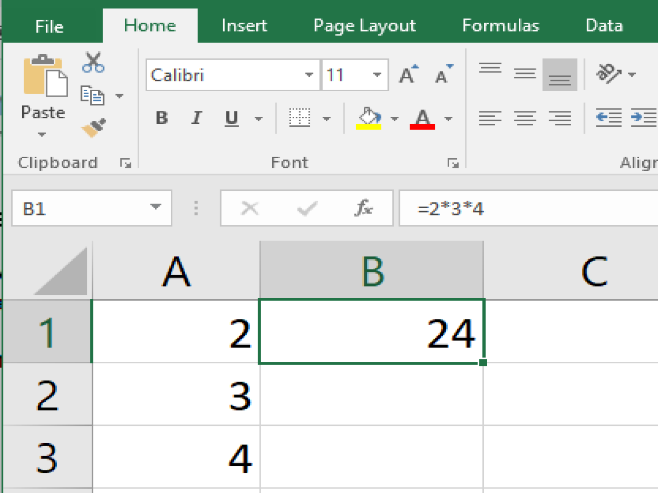
We have the given numbers of 2,3 and 4.
We picked B1 as our cell location where we want our product to be calculated.
We start the formula by = then the given number 2,3 and 4 and our separator for each given number is the sign ( * ) which is also our operator.
We are doing the right thing if we have entered in a finished formula of =2*3*4 on our excel spreadsheet. The result should come out as 24
It refers to the cell address of value on the spreadsheet, It is a combination of the column and row where the cell is located for Example A1 is located in column A and rows 1 so our cell reference is whatever value that is placed on A1.
It is a lot better to use a cell reference in a formula, you just click the cell or range of the one we want to perform the multiplication on and separate them by an ( * ) which is the symbol for multiplication on excel spreadsheet.
And rather than typing cell reference you can just navigate your mouse and click on that certain cell you want to get the product of, It eliminates the high probability of errors done by typing in the wrong cell reference.
As you can see in the example below, we have the put the numbers of 5,6 and 7 into cells and we chose B2 as our product cell location.
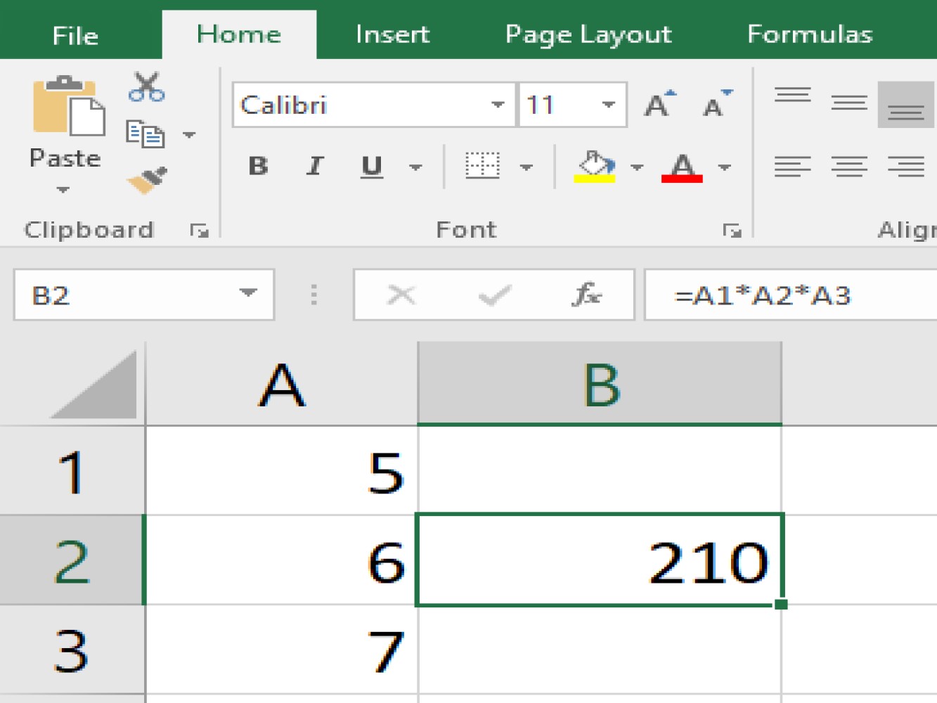
Start off the formula by typing = then drag the mouse to A1 where the value of 5 located.
Then press Shift + 8 for the keyboard shortcut on asterisk or if you have a numeric keyboad just press the asterisk sign ( * ) which is located in the middle of forward slash sign ( / ) and the minus sign ( - ).
Then click on A2 where the second value is located type another asterisk ( * ) then the last cell reference which is A3.
You should have the formula=A1*A2*A3 and then hit Enter and the result is 210.
TAKE NOTE
When you use a cell reference in a formula the answer or value of the product can be changed by simply changing the given numbers we wish to multiply.
This article concludes the things we need to know and to consider before performing multiplication in an Excel sheet. We have also discuss more methods to use Excel formulas to multiply in Part 2 of this tutorial. We hope you'll stick around.
/
ID: 61
Title: How to Use Excel Formulas Multiply (Part 1)
Meta Description: A demonstration of how to use Excel formulas to multiply values.
Meta Keywords: excel formulas multiply
Author: Data Pilot
Template: Unstructured Tutorial
Categories: Excel
Tags: Excel
Status: Published
/
We are going to enumerate different methods we can use to multiply using excel formulas, let us site examples on each method to make sure we cover everything about how to use multiplication in excel.
Before we go ahead and discuss multiplication let us first understand the different symbol of mathematical operators in Excel.
| Operation | Symbol |
|---|---|
| Addition | + |
| Subtraction | - |
| Multiplication | * |
| Division | / |
Now we know the mathematical operators of Excel formulas we can go ahead on focus on our topic which is multiplication which in Excel we use with the (*) the asterisk symbol
It is much easier if you have a keyboard with numeric keypad, If not, the multiplication symbol (*) asterisk can easily be typed under keyboard shortcut Shift + 8
Before we proceed with the example I would like to put EMPHASIS on excels Order of Operations which is also known as PEMDAS which is an abbreviation of Parentheses, Exponentiation, Multiplication, Division, Addition or Subtraction.
Note: On the PEMDAS for multiplication, division, addition, and subtraction it does not matter which comes first in the order, but not for the parentheses and exponentiation.
We have different methods in excel where we can perform multiplication, Let us enumerate them in this article and we can start off with.
The simplest way to do the multiplication operation is by multiplying your 2 or more given numbers ( which is called Multiplier and Multiplicand in Math terms ) on the cell you want your answer ( Product ) to appear.
TAKE NOTE:
Let us site an example where excel formulas multiply in numbers using asterisk can be used:
We have the given numbers of 2,3 and 4.
We picked B1 as our cell location where we want our product to be calculated.
We start the formula by = then the given number 2,3 and 4 and our separator for each given number is the sign ( * ) which is also our operator.
We are doing the right thing if we have entered in a finished formula of =2*3*4 on our excel spreadsheet. The result should come out as 24
It refers to the cell address of value on the spreadsheet, It is a combination of the column and row where the cell is located for Example A1 is located in column A and rows 1 so our cell reference is whatever value that is placed on A1.
It is a lot better to use a cell reference in a formula, you just click the cell or range of the one we want to perform the multiplication on and separate them by an ( * ) which is the symbol for multiplication on excel spreadsheet.
And rather than typing cell reference you can just navigate your mouse and click on that certain cell you want to get the product of, It eliminates the high probability of errors done by typing in the wrong cell reference.
As you can see in the example below, we have the put the numbers of 5,6 and 7 into cells and we chose B2 as our product cell location.
Start off the formula by typing = then drag the mouse to A1 where the value of 5 located.
Then press Shift + 8 for the keyboard shortcut on asterisk or if you have a numeric keyboad just press the asterisk sign ( * ) which is located in the middle of forward slash sign ( / ) and the minus sign ( - ).
Then click on A2 where the second value is located type another asterisk ( * ) then the last cell reference which is A3.
You should have the formula=A1*A2*A3 and then hit Enter and the result is 210.
TAKE NOTE
When you use a cell reference in a formula the answer or value of the product can be changed by simply changing the given numbers we wish to multiply.
This article concludes the things we need to know and to consider before performing multiplication in an Excel sheet. We have also discuss more methods to use Excel formulas to multiply in Part 2 of this tutorial. We hope you'll stick around.
Here's the links for each part of the article: