In this article we'll discuss and go over an example of what the Excel Index function does, when to use it, and the syntax. This is a very commonly used function in Excel and therefore is good to know this function by heart. The Excel index function returns the value of a cell given a range and a specified row and column.
The excel index function is very useful if you want to get the value of a given position in the table using the indexes of the rows and columns while identifying the range of the specified value. Look for the example below:
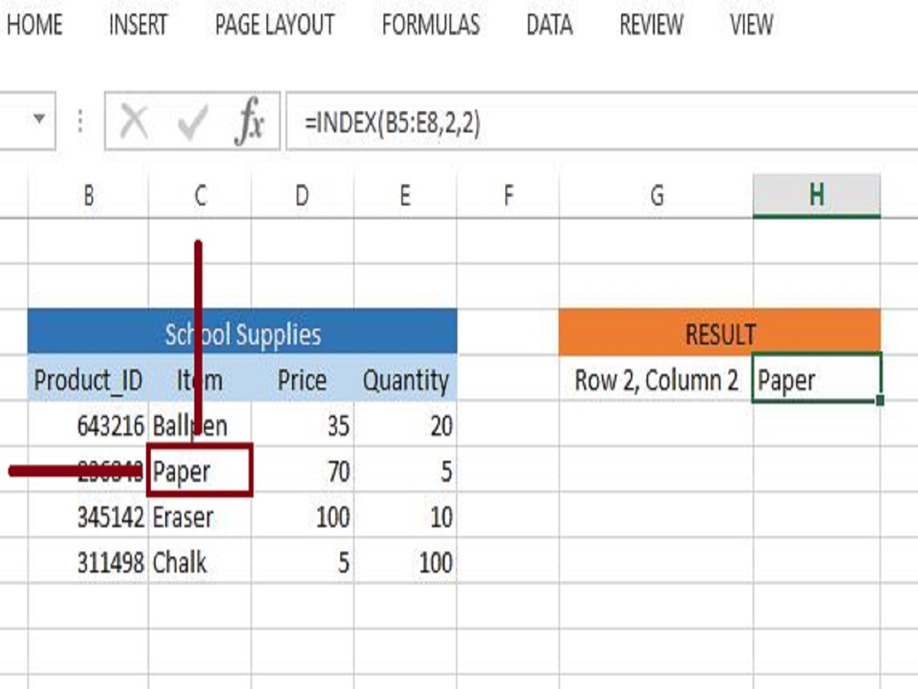
The image shown above has a result value of paper in cell "C6" after using the index function because we pinpoint the intersection of the value by defining the table with a position of the second cell in a row and also the second cell in a column in the worksheet of the selected range of cells in "B5:E8".
Let's define the three arguments used in our example:
We can also use the index function by using the built-in library of Microsoft Excel.
On the FORMULAS tab look for the "Function Library" group and click on the button Lookup & Reference then it will display a drop-down menu of all the functions with a lookup category with many options. Lastly, select the INDEX function.
You will be given a selection of arguments using an array type or reference type.
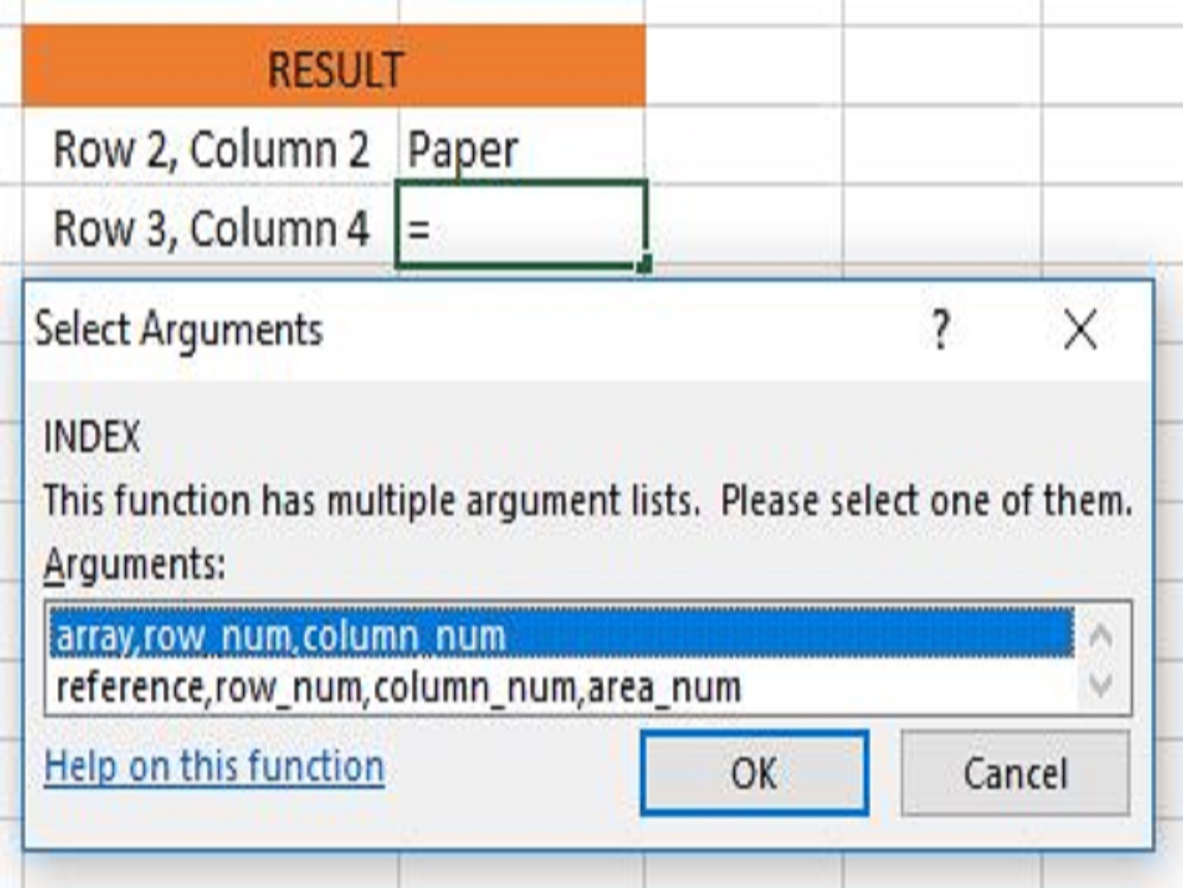
Let's try using the array type of the index function for the second example:
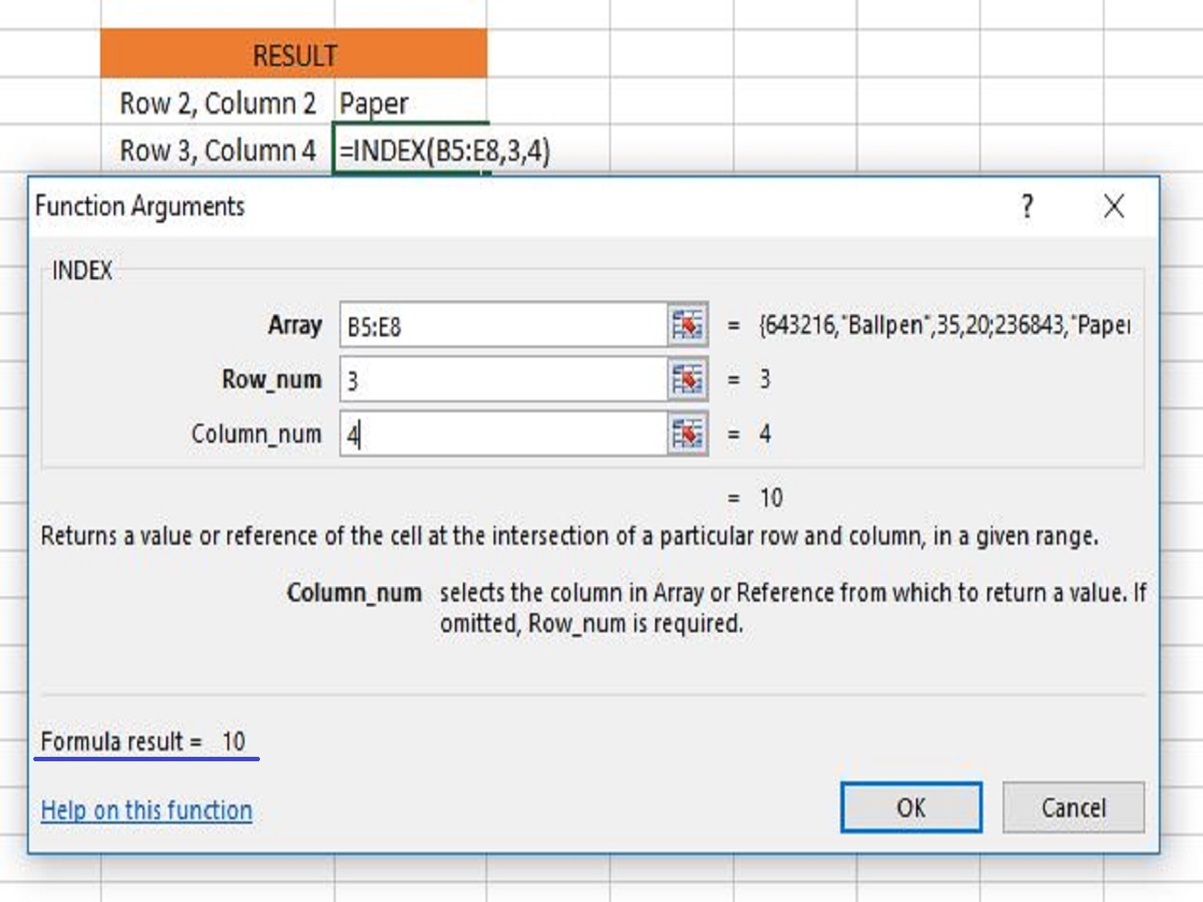
We specify the cell B5:E8 because it will be the range of objects of the array inside our table in the worksheet followed by the row number and column number. After putting all of the positions you want to display, the function automatically shows the result of the formula on the intersection of the cell in row 3 and cell in column 4.
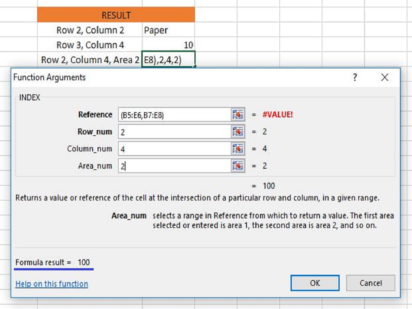
Next is the reference type in the index function for our next example:
We create the cell reference in two areas by selecting the first one (cell reference from B5 to E6) and the second (cell reference from B7 to E8).
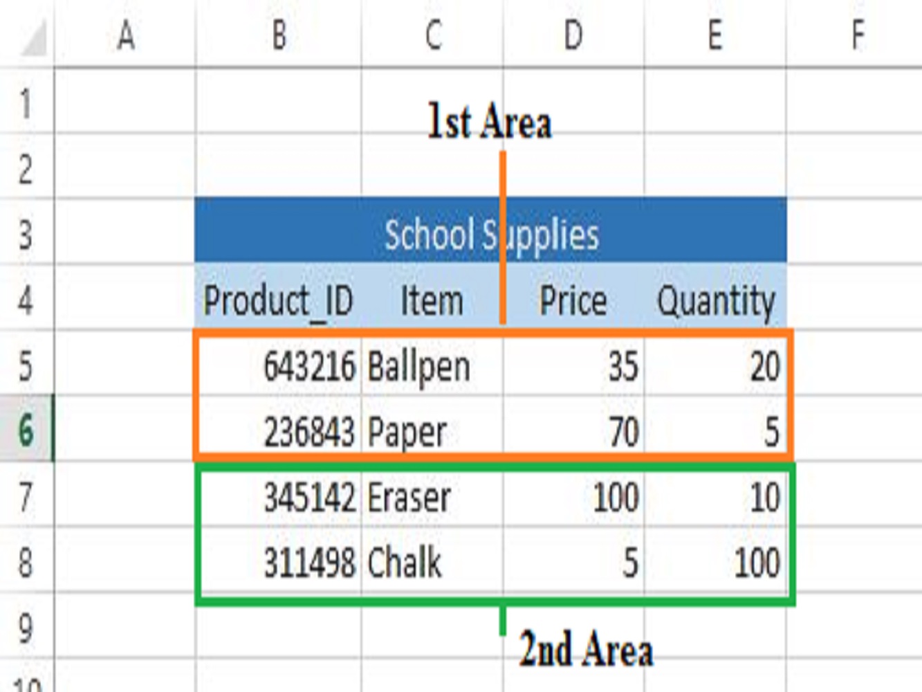
Next, to specify the position of the row and column number and select which area you want the index function to return the value. It also shows the result of the formula automatically on the intersection of the row and column before clicking on the OK button.
Now you have learned and use the index function which locates the column and row value of the table in the worksheet in Excel and retrieve an output depends on the given index.
This article concludes the tutorial on using the index function syntax in Excel and the formula for the array type and reference type. This function is a great building block for more complex formulas and calculations that you'll want to perform in Excel. Thanks for joining us for this article on the Excel INDEX function.