Introduction

This article is a tutorial that will discuss how to use the Excel rank function to organize the list of data. We'll quickly go over some basic prerequisites and then jump into exactly what the rank function does. Let's jump in!

Prerequisites

You need Microsoft Excel installed on your device.
A basic knowledge in Text function is required to understand the right function's usage.

Excel rank function

As compared to a list of other numeric values, the Excel RANK function returns the rank of a number value. Through the use of an optional order argument, RANK will level values from largest to smallest, and even from smallest to largest.

The Rank function syntax is:

=RANK(number,ref,[order])

The required argument:

• number - This would be the value in which we find a rank.
• ref - An array of numbers, or reference to, number of list. The Non-numeric values are ignored in ref argument.

The optional argument:

order- It is a number that specifies how the ranking would be carried out. It can be ascending or descending order.

• 0- Number of ranks as if the ref was a number sorted in descending order.
• 1 - When the order is any value other than zero, this ranks numbers as if the ref was a list sorted in ascending order.

When we omit the argument a default value of 0 will be used.

Rank function examples

When you give a number and a list of numbers to the RANK function, this will ask you the rank of a number in the list, either in ascending or descending order.

To demonstrate the rank function in Excel, let's use an example:

To find a rank of the first cell, enter the following formula:

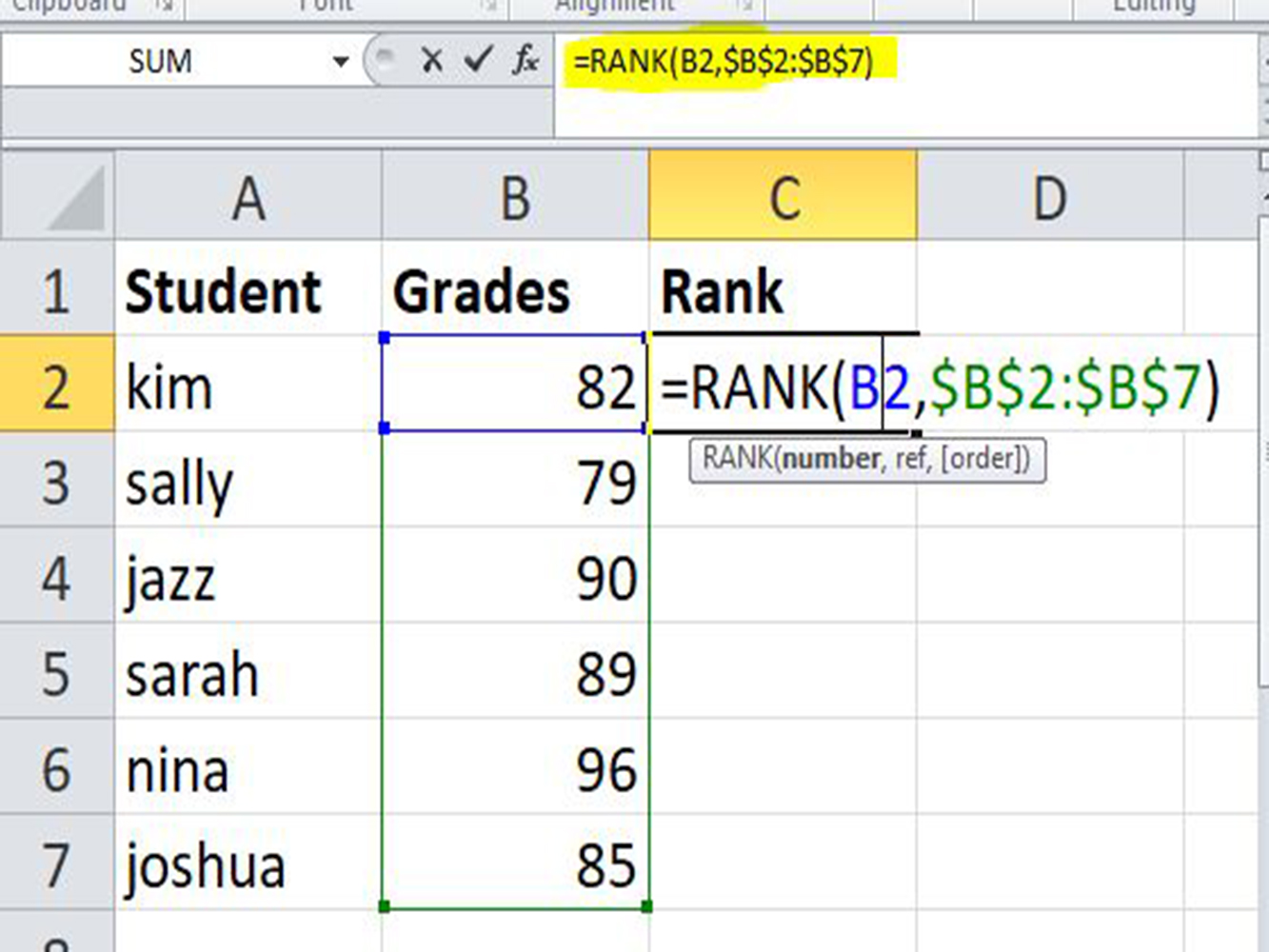
In the table above, there is a list of students and their corresponding grades in cell B2;B7.

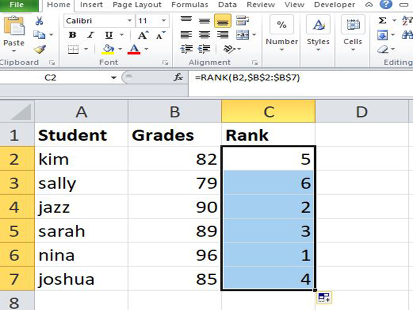
Drag down to copy the formula to the remaining cells. The grades will be ranked in descending order.

Excel rank function order

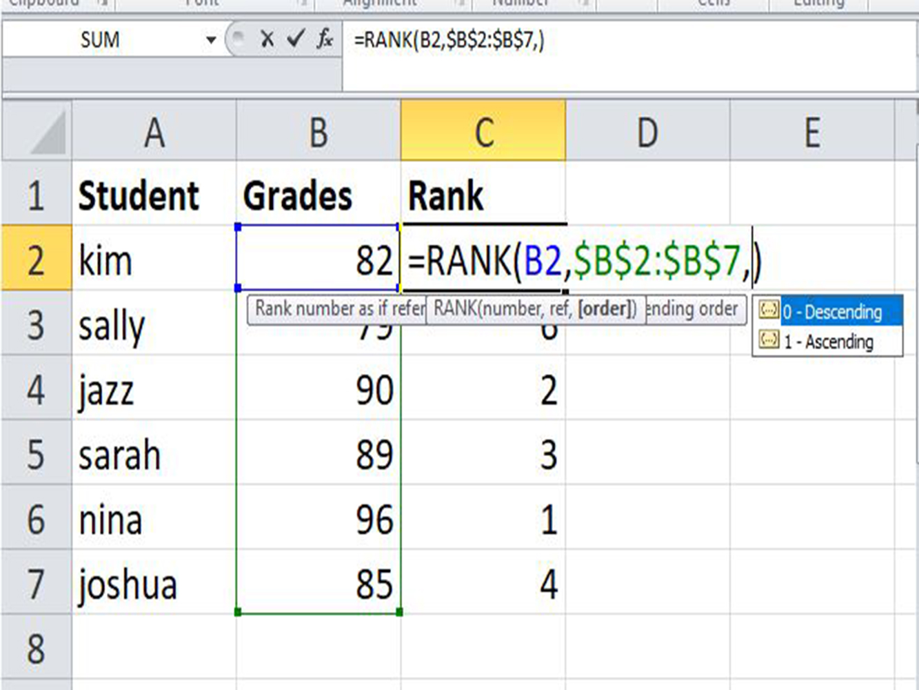
In the syntax of the rank function, the order is optional. This argument will ask you whether to rank the list in descending or ascending order.

To rank in descending order

If you choose the 0 in the order option, or even the order argument is omitted, the rank will be set in descending order.

For example:

The largest value ranked to 1 and the smallest value gets the rank of 6.

To rank in ascending order

When you are using a 1 as the order set, or if you insert any number other than zero as the order argument then, the rank gets set in ascending order.

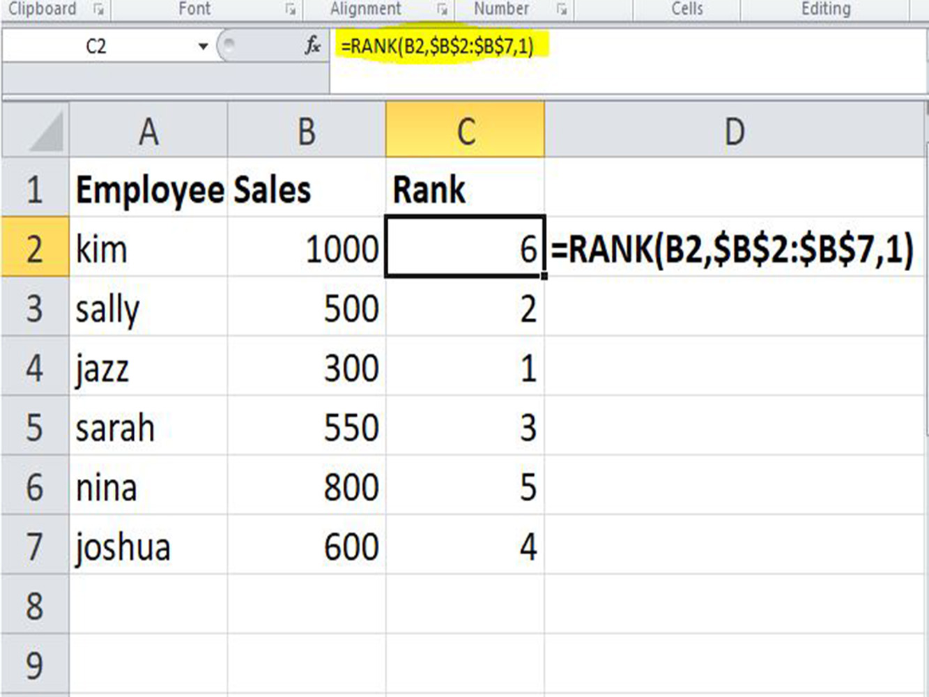
The largest value ranked to 6 and the smallest value gets the rank of 1.

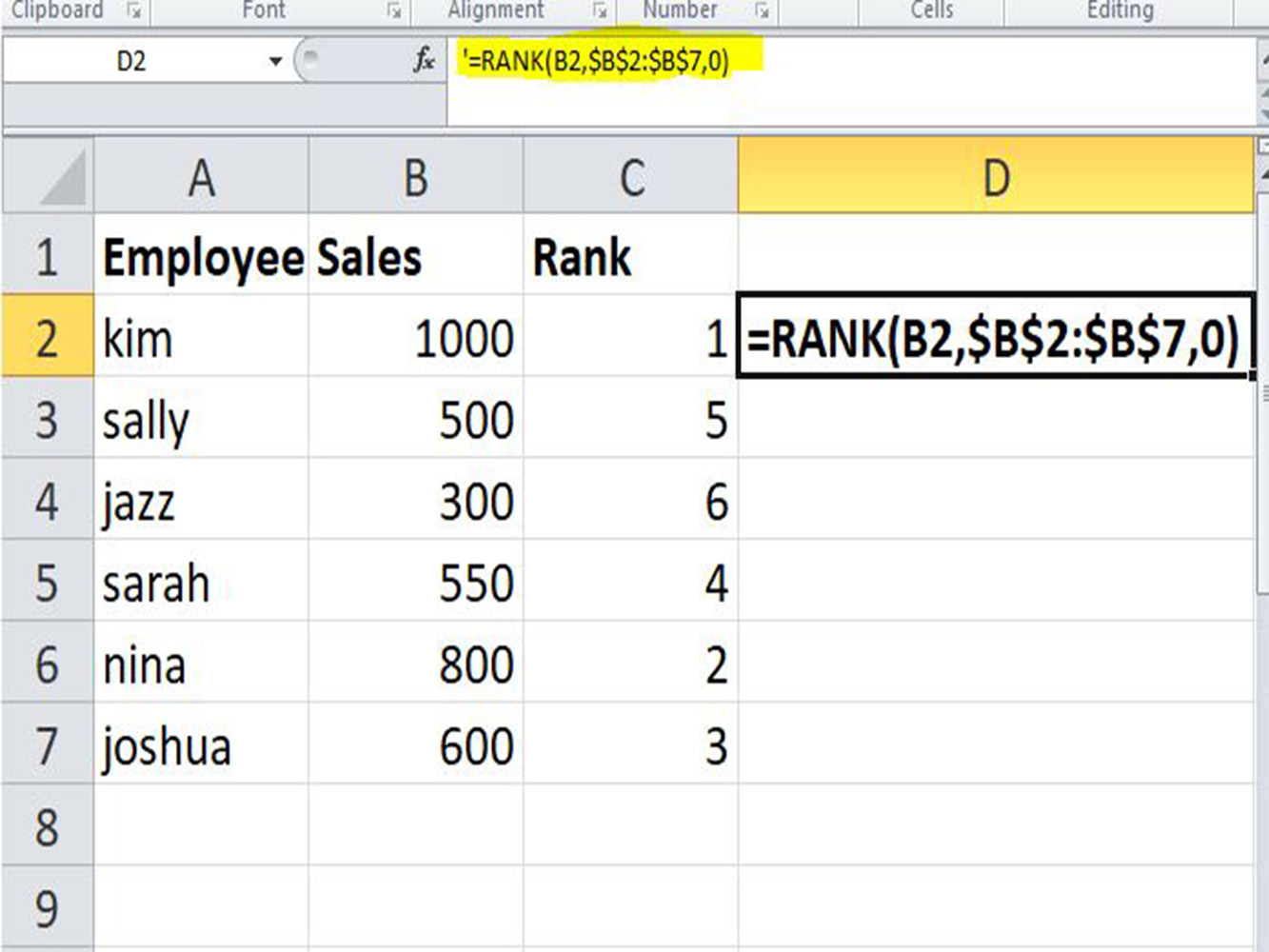
To make your formula flexible, you can type the order argument in any cell it could be 0 or 1 as a cell reference.

For example, type the 1 in cell D2 then, link it as an order argument.

Note: Use an absolute reference ($D$2) before you drag down the formula because if you use the relative reference (D1) it won't retain the same value and each rows value will be changed.

Conclusion

We have covered what the Excel RANK function does and the syntax to use it and change the options so you can rank in ascending in or descending order. We hope this tutorial helped you find your way to a better and more efficient Excel worksheet!