Introduction

In this second part of the article we will discuss further the total net income excel budget template we created in the first part. We'll be building upon it so make sure you've read part 1. You can find part 1 of the article here.

Prerequisites

Make sure that you have read the first part of this series article that creates an excel budget template example in your spreadsheet for us to know the total gain within a month of expenses.

Select the Total Income and Expenditure of the Example in the Spreadsheet

The cell 'B2' will represent the total amount of income within the month of January and we will reference the value in the cell 'B11', just use the formula like this: '=B11' on the cell 'B2'.

Next is the cell 'B3' that will have the total expenditure on the month of January. Just follow the given instructions a while ago.

Lastly copy the formula and paste it along the other month columns and the NET TOTAL will be the gain per month or the excess money you have.

Get the Total Income and Expenses in a Year

If you want to get the total amount of income and expenses with the net total value in a year, follow the instructions below :

On the last column of your month cell, create a new column with a TOTAL name.

Below the total, we will create the sum function to add all of the income from January to December.

=SUM(B2:M2)

The same goes for the expenditure row.

=SUM(B3:M3)

And the net total of the income and expenditure within the year would be the difference between the two.

=N2-N3

Modify the Budget Template in Excel for a Better Readability

First is to put a dollar sign to all of the numbers in the spreadsheet, just select the cells that contain a number and in the HOME tab look for the group Number then click on the dollar sign or any currency that you want to put.

Next is to select the month table from January to Total column then put some fill color and color of the font to make your table looks better.

Do the same with the income table and expenditure table.

Use the Conditional Formatting to Filter the Data

On your net total, we want to highlight the amount if it has greater than '$1250' and less than '$1180' from the month January to December.

Go to the HOME tab and look for the styles group, then you will see a button Conditional Formatting, when you click the button, a drop-down menu will show and choose the Highlight Cell Rules option followed by the greater than.

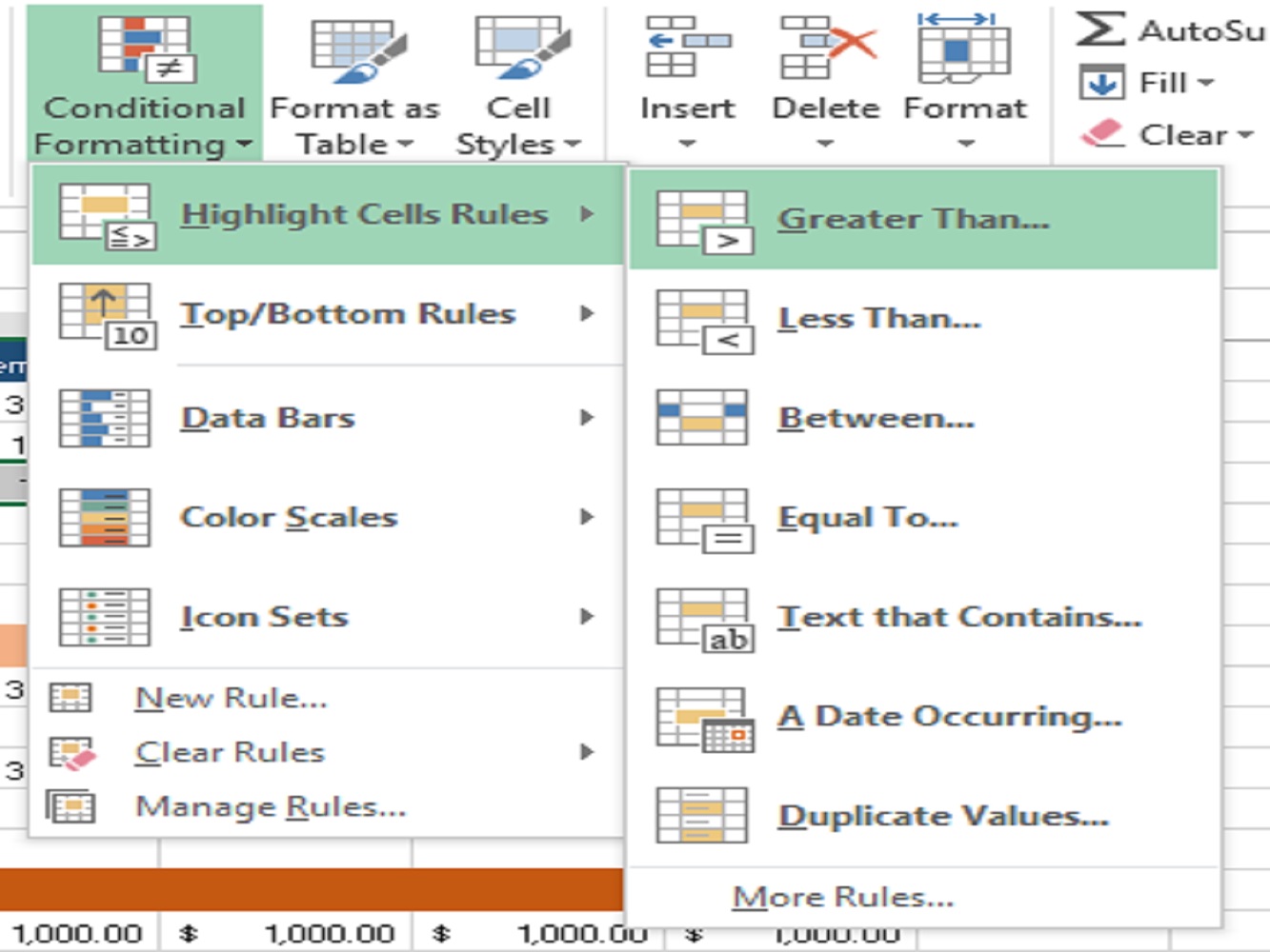
Just do the same with the less than value but change the color so that you can monitor the difference of the highlighted amount that is less than.

Conclusion

This article concludes the last part of creating an Excel budget template that also uses conditional formatting to highlight the amount of the month which has the greater than value or less than value.